Statistics Concepts¶

Statistics is the sister discipline to probability in mathematics. Statistics addresses the inverse problem of learning about probability distributions from data, as opposed to the forward problem of generating data from probability distributions. The term statistic is also a definition – a statistic is a “mathematical calculation of some data”. Since inference on probability distribution parameters relies upon statistics, the term Statistics is an appropriate name for the discipline.

PDFs and CDFs¶

As we have seen, there are two types of probability distributions:

Discrete distributions define positive probabilities for specific outcomes \(x\) of a discrete-valued random variable \(X\) that are defined using a probability mass function (PMF), i.e.,

\[Pr(X=x)\]

Continuous distributions on the other hand (perhaps unexpectedly and paradoxically) define \(Pr(X=x) = 0\) for every potential outcome \(x\) of a continuous-valued random variable \(X\) but define positive probabilities for \(Pr(X=x \in E \subseteq \mathbb{R})\) according to the area under the probability density function (PDF) \(\; f_X(X=x)\) over the set \(E\), i.e.,

\[Pr(X=x \in E) = \underset{E}{\int} f(X=x)\; dx\]

so that a PDF defines outcome prevalence in a relative (rather than absolute, i.e. probability) manner. For example, if \(f(X=x_1) = 2f(X=x_2)\) then in the long-run \(x_2\) will occur twice as frequently as \(x_1\). For more explanation, see this video about PDFs from Khan academy.

Note

EXERCISE

Have a look at the documentation for the probability distribution functionality in SciPy, which shows how to work with probability distributions using Python. Specifically, it shows how to use Python to evaluate probability mass functions and probability density functions – something we haven’t done yet. For example, here’s how to evaluate the density of the gamma distribution for a given outcome:

>>> from scipy import stats
>>> gamma_rv = stats.gamma(a = 5, scale = 10)
>>> gamma_rv.pdf(10)
0.0015328310048810102
>>> poisson_rv = stats.poisson(mu=20)

Once you’ve gotten the hang of this for the gamma distribution, try to generate analogous values for a Poisson distribution. If you’re running into trouble, consider what method of a poisson_rv object you should be calling. (Hint: should a Poisson random variable have a probability density function?). Once you’ve got that working, what would you say is the biggest difference between these values as associated with the gamma distribution compared to the Poisson distribution?

Both discrete and continuous distributions satisfy the axioms of probability, e.g.,

\(0 \leq Pr(X=x) \leq 1\) and \(0 \leq \underset{E \subseteq \mathbb{R}}{\int} f(X=x)\; dx \leq 1\)

\(\sum_{x \in S_X} Pr(X_i=x) = 1\) and \(\int_{-\infty}^{\infty} f(X_i=x) \; dx = 1\)

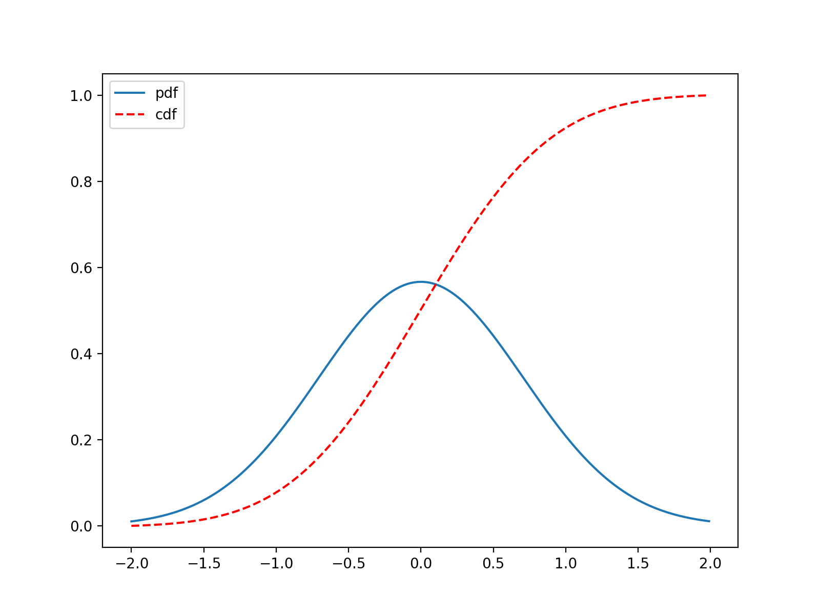
and both can be represented as a cumulative distribution functions (CDF), which is defined as

\[F_X(X=x) = Pr(X=x\leq x_0)\]

(Source code, png, hires.png, pdf)

Notice that for continuous distributions

\[F_X(X=x_0) = \underset{x<x_0}{\int} f(X=x)\; dx\]

which means that the derivative of the CDF is the the PDF

\[\frac{d}{dX}F_X(X) = f(X)\]

Note

QUESTION

Are you surprised that discrete and continuous distributions can BOTH be defined in terms of a CDF even though discrete distributions only have PMF and not a PDF and continuous distributions only have a PDF and not a PMF?

Expectation¶

The expectation operator for a random variable \(X\) is defined as

\(E[X] = \displaystyle \sum_{x\in S_X} x Pr(X=x)\)

\(E[X] = \displaystyle \int_{-\infty}^{\infty}x f_X(x)dx\)

for discrete and continuous distributions, respectively.

Parameters¶

Recall the first through fourth distributional moments mentioned previously. The first moments is the above expectation \(E[X]\) or mean of the distribution and is a measures the central tendecy of the distribution. For more explanation, see this video about random variables from Khan academy.

Note

EXERCISE

The second (central) moment of a distribution – the variance – is a measure of spread of the distribution and is defined as

\[Var[X] = E\left[(X-E[X])^2\right]\]

and the standard deviation, which is defined on the original units of the random variable is defined as \(\sigma_X = \sqrt{Var[X]}\).

How would you actually calculate the standard deviation of a random variable with a given discrete distribution, \(Pr(X=x)\)?

For more information, see: Measures of spread (Khan academy).

Joint Distributions¶

When we’re talking about random variables, we don’t use the set notation that we did for events, e.g., \(A \cap B\). Instead, we specify the distribution associated with two random variables \(X_1\) and \(X_2\) as \(P(X_1, X_2)\) where \(P\) specifies either a PMF or a PDF. A distribution such as this that is specified for two or more random variables is called a joint distribution. And further, the joint distribution of a collection of random variables \(X_i, \; i = 1, \cdots, n\) is defined by the distributional form of the chain rule which is

\[\displaystyle P\left(X_1, X_2, \cdots X_n\right) = \left(\prod_{i=2}^{n} P\left(X_i | X_{i-1}, \cdots X_1 \right)\right) \times P\left(X_1\right)\]

Further, just as with events, if the \(X_i\) are independent of each other then

\[\displaystyle P\left(X_1, X_2, \cdots X_n\right) = \prod_{i=1}^n P\left(X_i\right)\]

Note that the the mathematical multiplication notation \(\displaystyle \prod_{i=1}^{n} c_i\) for numbers \(c_i, i = 1, \cdots, n\) is just like the mathematical summation notation \(\displaystyle \sum_{i=1}^{n} c_i\) except that the \(c_i\) are multiplied together instead of being added together.

Note

EXERCISE

Write out the distributional chain rule defining \(P\left(X_1, X_2, X_3, X_4, X_5\right)\) and give an account of how it might be interpreted. E.g., “First we caclulate the probability of \(X_1\)…”

Linear Association¶

Linear association between two variables is encoded as the covariance of the joint distribution of those two variables

\[ \begin{align}\begin{aligned}Cov[X,Y] &= E[(x - E[X])(y - E[Y])]\\ &= \left[\underset{x,y \in S_X,S_Y}{\sum or\int}\right] (x - E[X])(y - E[Y])P(X=x,Y=y) \left[dxdy\right]\end{aligned}\end{align} \]

where the brackets simply indicate appropriate notational usage depending on if we’re talking about discrete or continuous random variables.

Much like with standard deviation, it can be helpful to be on a more natural scale, so we often use correlation (which varies from -1 to +1 with 0 indicating “no linear association”) rather than covariance (which is measured on the product of the two variables unit) – to describe the strength of a linear relationship:

\[Corr[X,Y] = \frac{E[(x - E[X])(y - E[Y])]}{\sigma_X\sigma_Y} = \frac{Cov[X,Y]}{\sigma_X\sigma_Y}\]

Marginal Distributions¶

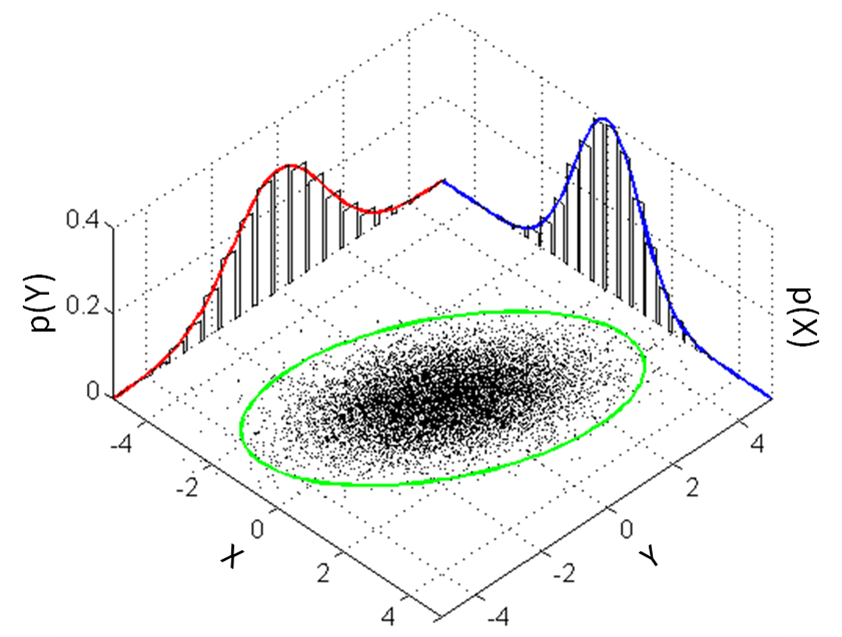
We have seen marginal distributions already – they are simply distributions of a single random variable. However, recasting the Law of Total Probability in terms of random variables \(X\) and \(Y\), we have for

discrete distributions

\[\displaystyle Pr(X=x) = \sum_{y \in S_Y} Pr(X=x, Y=y) = \sum_{y \in S_Y} Pr(X=x|Y=y) Pr(Y=y)\]

continuous distributions

\[\displaystyle f(X=x) = \int_{y \in S_Y} f(X=x, Y=y) \;dy = \int_{y \in S_Y} f(X=x|Y=y) f(Y=y) \;dy\]

which shows how marginal distributions \(Pr(X=x)\) and \(f(X=x)\) can be derived from their higher order joint distributions \(Pr(X, Y)\) and \(f(X, Y)\), respectively. Thus, a marginal distribution of a (possibly not independent) multivariate (joint) distribution is just the distribution of a single dimension (random variable) of the multivariate (joint) random variable. Marginal distributions are the unpacked variables of joint distributions.

So, while the chain rule allows us to build up joint distributions from conditional (“marginal”) distributions, the law of total probability allows us to unpack joing distributions into marginal distributions.

Note

EXERCISE

Draw the above plot, labeling it with all the concepts we’ve covered so far.

Statistics¶

Statistics are often chosen for their correspondence to specific distributional parameters for the purposes of estimating those parameters. It’s important to always remember the distinction between statistics and parameters, though: statistics are numerical calculations that use sample data for their calculation, while parameters are mathematical manipulations carried out on distributional forms.

A statistic that corresponds to the population mean is, unsurprisingly, the sample mean:

\[\bar{x} = \frac{1}{n}\sum_j^n x_j\]

However, alternative statistics with different robustness and behavior profiles, such as sample median and the sample mode, are available for measuring centrality. The statistic that corresponds to the population variance is the sample variance:

\[s^2 = \frac{1}{n-1} \sum_j^n (x_j - \bar{x})^2\]

But again, alternative statistics such as the range and inter-quartile range are available for measuring spead. And of course, the sample standard deviation \(s = \sqrt{s^2}\) is much easier to interpret than the sample variance.

There are a couple common choices for statistics that correspond to linear associations parameters. The Pearson correlation coefficient measures the linear relationship between two datasets. The alternative Spearman correlation is a nonparametric measure of the monotonicity of the relationship between two datasets, which is just a fancy way of saying that calculates the correlation on the ranks rather than original values. Here’s how you can calculate these statistics using Python:

>>> from scipy.stats import pearsonr
>>> from scipy.stats import spearmanr
>>>
>>> pearsonr([1,2,3,4,5],[5,6,7,8,7])
(0.83205029433784372, 0.080509573298498519)
>>> spearmanr([1,2,3,4,5],[5,6,7,8,7])
(0.82078268166812329, 0.088587005313543812)

The first value in the above tuples is the correlation. The second is a p-value of a statistical test of the null hypothesis of no association. The two tests are based on different distributional assumptions and as such are, unsurprisingly, different. A spurious relationship is a relationship is said to exist between two or more random variables that are not causally related to each other but have a relationship due to a common confounding factor.

A Warning¶

Confounding is just one of the many difficulties that will need to be dealt with in real data. When you actually begin working with real data you’ll see that things can be quite messy. In fact, messy would be an understatement for some outliers that will be present in your data. These outliers can drastically affect your calculated statistics and hence your conclusions. Weary and vigilant attention is required to suss out these influential data points and decide what is to be done about them. And what if you have missing data that’s not even available to look at? Will you impute the missing data? If so, with how much sophistication? Or will you simply disregard samples with missing entires? As you can see, there are many questions and, unfortunately, very often too few answers…

Note

EXERCISE

List out some statistics you could calculate with the data in the above plot that you drew.

Further study¶

Most major statistical textbooks, for example (the free) Elements of Statistical Learning will begin with an overview of the topics in this section.