Probability Distributions
A probability distribution is a mathematical formalization that describes a particular type of random process.
Properties of Distributions
Probability Distributions are classified into two categories:
discrete – producing outcomes that can be mapped to the integers (such as 1, 2, …)
continuous – producing real-valued outcomes (such as 3.14… or 2.71…)
Discrete distributions are specified using probability mass functions often indicated as \(Pr(X=x)\) while continuous distributions are specified using probability density functions often indicated as \(f(X=x)\).
Discrete distributions specify probabilities of observing outcome \(x\) from a discrete random variable \(X\) directly, while continuous distributions specify the behavior of realizations \(x\) of a continuous random variable \(X\) in a retaliative rather than absolute manner. For example, if \(f(X=x_1) = 2f(X=x_2)\) then in the long-run \(x_2\) will occur twice as frequently as \(x_1\).
Regardless of whether or not a random variable \(X\) is discete or continuous, if it is distributed according to a distribution named \(XYZ\) with parameters \(\alpha\) and \(\beta\), and so on, then we write
and if a collection of \(n\) random variables \(X_i, \; i=1, 2, \cdots n\) are identically and independently distributed (i.i.d) —i.e., the random variables have the same distribution and the realization of one does not influence the realization of another— then we write
For both continuous and discrete distributions, there are four properties – the first through fourth moments – that are often used to describe a distribution:
Expectation (or Mean) characterizes the location of a distribution
Variance or Standard Deviation (square root of the variance) characterizes the spread of a distribution
Skewness characterizes the asymmetry of a distribution
Kurtosis characterizes the heavy-tailedness of a distribution (i.e., how ofter extreme outlier events occur under the distribution.
Essential Discrete Distributions:
Bernoulli
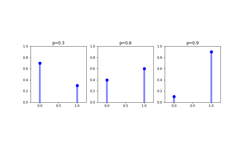
A Bernoulli distribution is a discrete probability distribution modeling a one chance attempt that results in either a success of a failure. Such an attempt is called a Bernoulli trial, with a success typically recorded as a \(1\) and a failure typically recorded as a \(0\). The most commonly cited example of a Bernoulli trial is getting a heads on a coin flip, where the chance of getting a heads is \(50\%\) if the coin is fair (but another probability otherwise). The probability mass function for a Bernoulli random variable \(X\) is defined as
where \(p\) is the parameter of the Bernoulli distribution and the mean and variance of the random variable \(X\) modeled using a Bernoulli distribution are, respectively
\(E[X] = p\)
\(Var(X) = p(1-p)\)
(Source code, png, hires.png, pdf)

Note
CLASS DISCUSSION
Let’s say that I polled all first graders in the state of colorado and asked the question do you like/dislike your teacher. The answers are discrete values and the distribution of those answers could be modeled with a Bernoulli model. What are some other examples?
Check out this khan academy video on the Bernoulli distribution if you need some further intuition about Bernoulli distributions.
Binomial
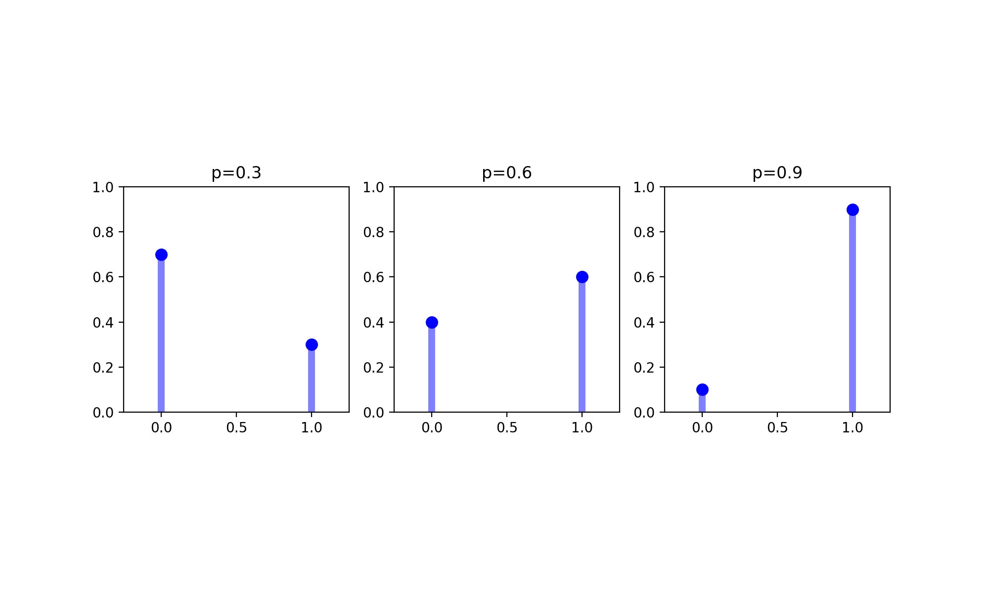
The binomial distribution is a discrete probability distribution that defines the probability of observing exactly \(k\) successes out of \(n\) identical Bernoulli trials. The probability mass function for a Binomial random variable \(X\) is defined as
where \(p\) and \(n\) are the parameters of the binomial distribution and the mean and variance of the random variable \(X\) modeled using a binomial distribution are, respectively
\(np\)
\(np(1-p)\)
(Source code, png, hires.png, pdf)
Note
CLASS DISCUSSION
The number of heads that come from flipping a coin 10 times is a discrete value that can be modeled with a binomial distribution. What are some other examples of random variables that might be modeled with a binomial distribution?
Check out this khan academy video on the binomial distribution if you need some further intuition about binomial distributions.
Poisson
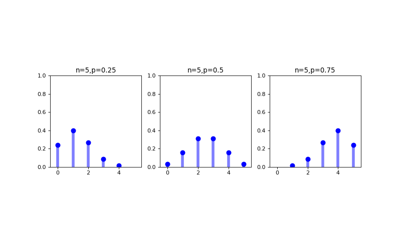
The Poisson distribution is a discrete probability distribution that can be used to model the number of times an event occurs within a given fixed time interval; specifically, it exactly defines a probability model for the number of arrivals of a sequential process of exponentially distributed time intervals in that window. (We will discuss the exponential distribution further below). (If all of that sequential process process stuff didn’t make any sense, don’t sweat it for now). The relationship of the Poisson distribution to the exponential distribution notwithstanding, the probability mass function for a Poisson random variable \(X\) is defined as
where \(\lambda\) is the parameter of the Poisson distribution and the mean and variance of the random variable \(X\) modeled using a Poisson distribution are, interestingly, the same:
\(E[X] = Var(X) = \lambda\)
(Source code, png, hires.png, pdf)

Note
CLASS DISCUSSION
The probability that one, two,… uber cars pass in front of my building in an hour is a discrete value that could potentially be modeled with a Poisson distribution. What are some other examples of random variables that could be modeled as using a Poisson distribution.
Bonus: Can any of these these examples be modeled using a binomial distribution?
Check out this How the Binomial and Poisson Distribution are Related (khan academy) video if you’re interested in learning a little bit more about the second question in the above exercise. Check out the Poisson distribution example (khan academy) video if you need some more intuition about Poisson distributions. And finally, some further example applications of the Poisson model are discussed here.
Essential Continuous Distributions:
Uniform
The (continuous) uniform distribution generates completely random occurrences over a defined space. The probability density function of the uniform distribution defined over an interval on the real line is specified as
where \(a\) and \(b\) are the parameters of the uniform distribution and the mean and variance of the random variable \(X\) modeled using a uniform distribution are, respectively
\(E[X] = \frac{a+b}{2}\)
\(Var(X) = \frac{(b-a)^2}{2}\)
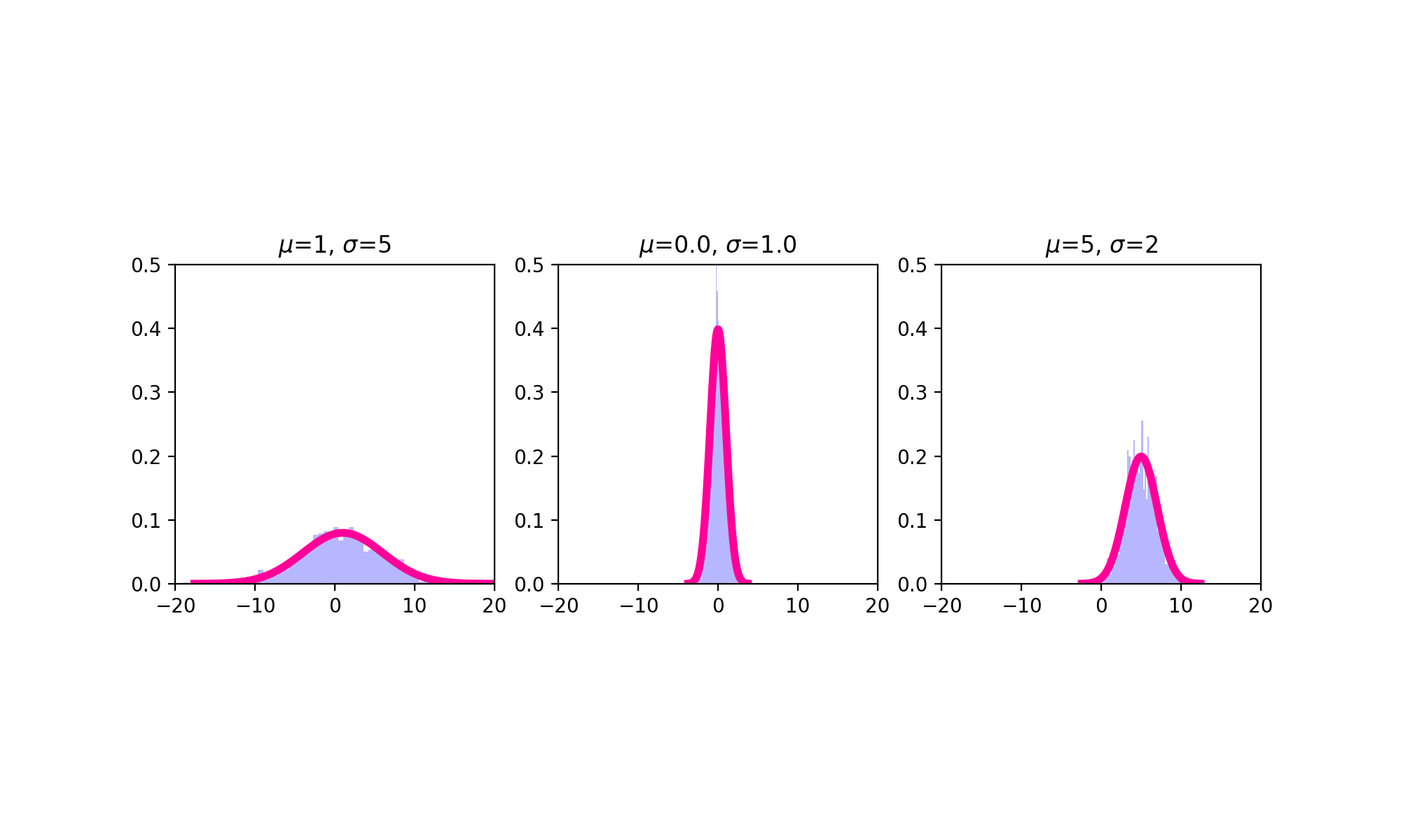
Normal/Gaussian
The Gaussian or normal distribution is a continuous probability distribution whose probability density function is defined as
where \(\mu\) and \(\sigma^2\) are the parameters of the normal distribution and the mean and variance of the random variable \(X\) modeled using a normal distribution are, respectively
\(E[X] = \mu\)
\(Var(X) = \sigma^2\)
The normal or Gaussian distribution is the distribution most frequently encountered in statistics. This is because there is a theorem (The Central Limit Theorem, or CLT) that, loosely speaking, says that random variables made up of sums of other random variables tend to be normally distributed. And since many random variables in our world are in some regard composite variables in this manner, many of the variables in our world do appear to be (approximately) normally distributed. Another reason we come across the normal distribution so much in statistics is because the CLT phenomenon can be leveraged as part of hypothesis testing. (We will cover hypothesis testing tomorrow).
(Source code, png, hires.png, pdf)
Note
CLASS DISCUSSION
Test scores, IQs, heights, finishing times from the Boston marathons have all been empirically shown to be (almost/approximately) normally distributed. Are you surprised to learn this?
Check out this khan academy video on the normal distribution if you need some further intuition about normal distributions.
Reparameterization
The way a distribution is parameterized is actually an arbitrary choice. I.e., there many ways way in which the parameters of a distribution could be be specified. For example, the inverse of the variance \(\tau = 1/\sigma^{2}\) is known as the precision in a normal distribution context and we could easily specify the Gaussian probability density function using the precision \(\tau\) rather than the variance \(\sigma^{2}\). For that matter, would you say that the Gaussian probability density function is specified in terms of the variance \(\sigma^{2}\), or the standard deviation \(\sigma\)?
Less Essential distributions:
Geometric
The geometric distribution is a discrete probability distribution that defines the probability of needing to perform \(k-1\) identical Bernoulli trials before a success is observed on the \(k^{th}\) trial. The probability mass function for a Geometric random variable \(X\) is defined as
where \(p\) is the parameter of the geometric distribution and the mean and variance of the random variable \(X\) modeled using a geometric distribution are, respectively
\(E[X] = \frac{1}{p}\)
\(Var(X) = \frac{1-p}{p^2}\)
Sometimes probabilities of the geometric distribution are given in terms of the number of failures (\(k-1\)) as opposed to the total tries (\(k\), as done above) involved in finally observing a success.
Hypergeometric
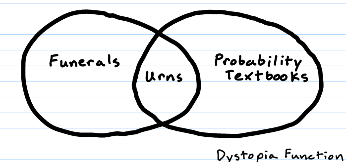
The hypergeometric distribution is a discrete probability distribution that defines the probability of \(k\) successes from a population of size \(n\) when sampling without replacement. To visualize this, think of an urn (“stats speak” for “jar”) containing two types of marbles – say, red and green – and define drawing a green marble as a success and drawing a red marble as a failure. The hypergeometric distribution then defines the probabilities of the number of marbles that will be green out of a total of \(n\) marbles sampled from the urn. The probability of \(k\) successes out of \(n\) attempts in this context are not binomially distributed because the probability of success on each subsequent sample changes based on what has been previously drawn out of the urn. Stated explicitly, the probability mass function for a hypergeometric random variable \(X\) is defined as
where \(N, K\), and \(n\) are the parameters of the geometric distribution specifying the size of the population, the total number of individuals in the population, and the number of individuals to be sampled for a given random variable experiment \(X\), respectively.
The hypergeometric distribution is very interesting because it allows the mean and variance of the random variable \(X\) to be independently specified through the parameters \(N, K\), and \(n\), as opposed to the binomial distribution which only allows one to specify a deterministic relationship between the mean and variance. Thus, the clear probabilistic interpretation notwithstanding, the hypergeometric distribution can also be used in a purely pragmatic manner to flexibly model count data that has a different mean and variance combination from those allowed by the binomial distribution. Thus, the hypergeometric distribution can essentially be viewed as the discrete distribution alternative to the normal distribution in contexts where you want to model counts rather than continuous values.
Note
CLASS DISCUSSION
Is there a fundamental difference in the deterministic relationships between the mean and variance as specified in the binomial distribution versus the Poisson distribution? Or are the relationships in some sense a similar type of restriction?
Note
PAIRED EXERCISE
Discuss with your neighbor why the formulas for the geometric and hypergeometric probability mass functions make sense.
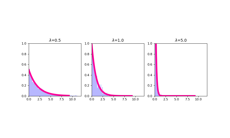
Exponential
The exponential distribution is a continuous probability distribution that has proven to be a useful model (with some deep theoretical justifications) for the distribution of “time to arrival” outcomes. Specifically, (as we have previously implicitly stated), the exponential distribution is the distribution of time to arrival outcomes for a so called Poisson process. Regardless, the probability density function for a Geometric random variable \(X\) is defined as
where \(\lambda\) is the parameter of the exponential distribution and the mean and variance of the random variable \(X\) modeled using an exponential distribution are, respectively
\(E[X] = \frac{1}{\lambda}\)
\(Var(X) = \frac{1}{\lambda^2}\)
The exponential distribution has an interesting “memoryless” property; namely, \(Pr(X \geq x+c |X \geq c) = Pr(X \geq x)\). What this actually means is that for any cutpoint \(X \geq c\), the re-normalized distribution looks exactly the same as an exponential distribution; only, it’s been shifted to the right by \(c\).
(Source code, png, hires.png, pdf)
Note
PAIRED EXERCISE
The exponential distribution is a special case of the gamma distribution. Another special case of the gamma distribution is the chi-squared distribution. Have one person explain the chi-squared distribution and the other explain the gamma distribution. Then together explain why the exponential and chi-squared distributions are special cases of the gamma distribution.
Note
EXERCISE
Have a look at the documentation for the probability distribution functionality in SciPy, which shows how to work with probability distributions using Python. Specifically, it shows how to use Python to generate random outcomes from probability distributions – something we haven’t done yet. For example, here’s how to generate random data from from the gamma distribution you learned about in the last exercise:
>>> from scipy import stats
>>> gamma_rv = stats.gamma(a = 5, scale = 10)
>>> gamma_rv.mean()
50.0
>>> gamma_rv.var()
500.0
>>> gamma_rv.rvs(10)
After you’ve tried using this code to sample gamma distributed random variables, try generating some samples from the other distributions. Play around the specifications of these distributions and see (a) how the mean and variance parameters of the random variables change and (b) how these characteristics are reflected in the random samples drawn from the distributions.
Note: the SciPy implementation of the gamma distribution uses the shape and scale parameterization rather than the shape and rate parameterization.
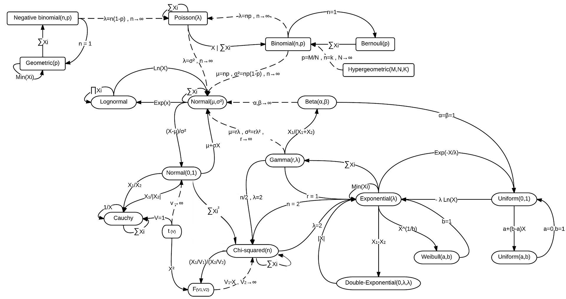
Distributional Relationships
We have already come across a couple connections that exist between different distributions (i.e., Bernoulli/Biomial, Binomial/Poisson, and Poisson/Exponential). Actually, there are many examples of such relationships that exist between probability distributions. And, unsurprisingly, there are many, many more distributions than the ones we covered here. Here is a diagram that suggests the scope of things here.
Data Modeling Considerations
Distributions can be used as models for your data! As such, there are a few standard considerations to keep in mind in assessing the appropriateness of a distribution as a potential data model:
Are my data discrete or continuous?
Are my data symmetric?
What limits are there on possible values for my data?
How likely are extreme values in my data?
Would my data reasonably look like a random sample from this distribution?