Statistical Inference
Statistics looks at some data, and asks the following questions:
Hypothesis Testing: how well does the data match some assumed (null) distribution?
Point Estimation: if not well, what instance of some distributional class does it match well?
Uncertainty Estimation: are there reasonable competitors to that best guess distribution?
Sensitivity Analysis: do our results rely heavily on our distributional assumptions?
These questions are addressed through various statistical/computational methodologies, e.g.,
- Numerical Optimization
Maximum Likelihood
Least Squares
Expectation Maximization (EM)
- Simulation of Null Distributions
Bootstrapping
Permutation Testing
Monte Carlo Methods
- Estimation of Posterior Distributions
Markov Chain Monte Carlo (MCMC)
Variational Methods
- Nonparametric Estimation
Bayesian Nonparametrics
Is my coin fair?
Hypothesis testing
Pose your question (“Is this coin fair?”)
Find the relevant population (“‘Flip results’ from this coin”)
Specify a null hypothesis \(H_0\) (“The chance of heads is 50%”)
Choose test statistic informing \(H_0\) (“The number of heads observed”)
Collect data (“Flip the coin \(n\) times”)
Calculate the test statistics (“Count the total heads flipped”)
Reject the null hypothesis if the test statistic looks “strange” compared to its sampling distribution under the null hypothesis; otherwise, fail to reject the null hypothesis
Simulating Data
import numpy as np
import matplotlib.pyplot as plt
import scipy.stats as st

n = 100
pcoin = 0.62 # actual value of p for coin
results = st.bernoulli(pcoin).rvs(n)
h = sum(results)
print("We observed %s heads out of %s"%(h,n))

We observed 67 heads out of 100
Null Hypothesis
p = 0.5
rv = st.binom(n,p)
mu = rv.mean()
sd = rv.std()
print("The expected distribution for a fair coin is mu=%s, sd=%s"%(mu,sd))

The expected distribution for a fair coin is mu=50.0, sd=5.0
Binomial Test
print("binomial test p-value: %s"%st.binom_test(h, n, p))

binomial test p-value: 0.000873719836912
Z-Test (with continuity correction)
z = (h-0.5-mu)/sd
print("normal approximation p-value: - %s"%(2*(1 - st.norm.cdf(z))))

normal approximation p-value: 0.000966848284768
Permutation (Simulation) Test
nsamples = 100000
xs = np.random.binomial(n, p, nsamples)
print("simulation p-value - %s"%(2*np.sum(xs >= h)/(xs.size + 0.0)))

simulation p-value - 0.00062
Note
EXERCISE
Does anyone know what a p-value is?
Hint: it is not the probability that the null hypothesis is false. (Why?)
Hint: it is not the probability that the test wrongly rejected the null hypothesis. (Why?)
Maximum Likelihood Estimation (MLE)
bs_samples = np.random.choice(results, (nsamples, len(results)), replace=True)
bs_ps = np.mean(bs_samples, axis=1)
bs_ps.sort()

print("Maximum Likelihood Estimate: %s"%(np.sum(results)/float(len(results))))
print("Bootstrap CI: (%.4f, %.4f)" % (bs_ps[int(0.025*nsamples)], bs_ps[int(0.975*nsamples)]))

Maximum likelihood 0.67
Bootstrap CI: (0.5800, 0.7600)
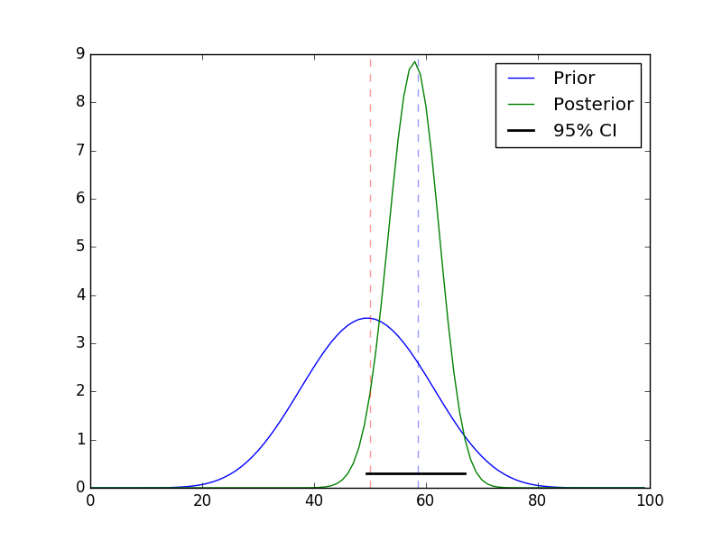
Bayesian Estimation
The Bayesian approach estimates the posterior distribution (i.e., the updated belief about the parameters given the prior belief and the observed data) and uses it to make point and interval estimates about the parameters. The calculations we demonstrate here have analytic solutions <https://en.wikipedia.org/wiki/Closed-form_expression>`_. For most real life problems the necessary statistical models are more complex and estimation makes use of advanced numerical simulation methods.
fig  = plt.figure()
ax = fig.add_subplot(111)

a, b = 10, 10
prior = st.beta(a, b)
post = st.beta(h+a, n-h+b)
ci = post.interval(0.95)
map_ =(h+a-1.0)/(n+a+b-2.0)

xs = np.linspace(0, 1, 100)
ax.plot(prior.pdf(xs), label='Prior')
ax.plot(post.pdf(xs), label='Posterior')
ax.axvline(mu, c='red', linestyle='dashed', alpha=0.4)
ax.set_xlim([0, 100])
ax.axhline(0.3, ci[0], ci[1], c='black', linewidth=2, label='95% CI');
ax.axvline(n*map_, c='blue', linestyle='dashed', alpha=0.4)
ax.legend()
plt.savefig("coin-toss.png")
Note
EXERCISE
Use the Python code above to play around with the prior specification a little bit. Does it seem to influence the results of the analysis (i.e., the resulting posterior distribution)? If so, how? How do you feel about that?
Note
CLASS DISCUSSION
Describe the role of Bernoulli and binomial distributions in our above example.
Describe the underlying hypothesis and the character of the tests assessing it.
Describe how the p-values are used to assess \(H_0\). (Hint: assume a significance level of \(\alpha=0.05\)).
Compare and contrast the Bayesian and Frequentist estimation paradigms.
Does anyone have other examples (not coin-flipping) where these tools might be applied?