Regression, Classification, Evaluation

Objectives

1. State assumptions of linear regression model

2. Estimate a linear regression model

3. Evaluate a linear regression model

Predictive Modeling

There are many circumstances in which we are interested in predicting some outcome \(Y\). To accomplish this task we set about collecting, selecting, and constructing data – a process referred to as feature engineering – that we think would help predict \(Y\). Given our selected features \(\textbf{X}\), the association between the features \(\textbf{X}\) and and the outcome \(Y\) can be expressed as

\[Y = f(\mathbf{X}) + \epsilon\]

where \(f\) explicitly describes the precise relationship between \(\textbf{X}\) and \(Y\), and \(\epsilon\) is…

Note

CLASS DISCUSSION

• What is \(\epsilon\)?

• How could we model \(\epsilon\)?

• How about \(f\)?

• Based on what you’ve seen so far, is Statistics and Probability more suited to describe \(\epsilon\) or \(f\)?

Types of Data

The data \(\textbf{X}\) that we use to predict \(Y\) can come in many varieties, i.e.

1. Continuous:

   • Price, Quantity, Sales, Tenure

   • Sometimes it makes sense to map to discrete variables

2. Categorical:

   • Yes/No, 0/1, Treated/Control, High/Medium/Low

   • Also called a factor

3. Missing Values

   • May require estimation

4. “Non-numeric”

   • Text, Audio, Images, Signals, Graphs

   • Requires transformation into meaningful quantitative features

Supervised Learning

Approximating \(f(\textbf{X})\) with some function \(\hat{f}(\textbf{X})\) in the face of noisy data (as a result of \(\epsilon\)) is known as model fitting. Actually, different disciplines have adopted different nomenclatures for this process.

Machine Learning	Notation	Other Fields
Features	\(\textbf{X}_{(n \times p)}\)	Covariates, Independent Variables, or Regressors
Targets	\(Y_{(n \times 1)}\)	Outcome, Dependent or Endogenous Variable
Training	\(\hat{f}\)	Learning, Estimation, or Model Fitting

Depending on the data type of the target, the supervised learning problem is referred to as either

• Regression (when \(Y\) is real-valued)

  E.g., if you are predicting price, demand, or size.

• Classification (when \(Y\) is categorical)

  E.g., if you are prediction fraud or churn

Data Size

• Associative Studies: test hypotheses

  • Association is causality under carefully controlled conditions

  • The power and accuracy of a test is an asymptotic function of \(N\)

• Predictive Studies: try to guess well

  • Complex models are prone to overfitting without sufficient \(N\)

  • Regularization limits overfitting and cross-validation assesses accuracy

Note

CLASS DISCUSSION

How would you differentiate Statistics and Machine Learning, if at all?

Unupervised Learning

When you’re not trying to predict a target \(Y\), but just seeking to uncover patterns and structures between the features \(\mathbf{X}\), the problem is referred to as Unsupervised Learning. The two primary areas of unsupervised learning are

• Clustering: e.g., hierarchical, k-means

• Dimension reduction: e.g., PCA, SVD, NMF

Linear Regression

Suppose that \(Y_i\) depends on \(X_i\) according to

\[Y_i = \beta_{0} + \beta_{1} X_i + \epsilon_i, \text{ where } \epsilon_i \overset{\small i.i.d.}{\sim}N\left(0, \sigma^2\right)\]

where \(\beta_{0}\), \(\beta_{1}\), and \(\sigma^2\) are the parameters of the model (intercept, coefficient and variance, respectively).

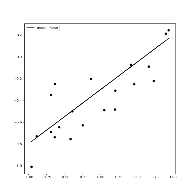
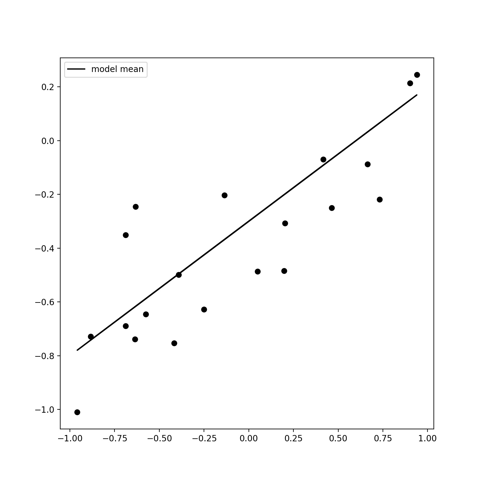
We can easily simulate some data under an instance of this set of models as follows:

import matplotlib.pyplot as plt
import numpy as np

def get_simple_regression_samples(n,b0=-0.3,b1=0.5,error=0.2):
    trueX =  np.random.uniform(-1,1,n)
    trueT = b0 + (b1*trueX)
    return np.array([trueX]).T, trueT + np.random.normal(0,error,n)

seed = 42
n = 20
b0_true = -0.3
b1_true = 0.5
x,y = get_simple_regression_samples(n,b0=b0_true,b1=b1_true,seed=seed)

fig = plt.figure(figsize=(8,8))
ax = fig.add_subplot(111)
ax.plot(x[:,0],y,'ko')
ax.plot(x[:,0], b0_true + x[:,0]*b1_true,color='black',label='model mean')
ax.legend()
plt.show()

(Source code, png, hires.png, pdf)

Note

QUESTION

If you added data into the plot above where could you add them that might be a cause for concern?

Note

CLASS DISCUSSION

If you increased to total number of data points generated by this model, how would the density of points in this picture look?

Now of course in real life you first get your data and then you estimate your model:

\[\mathbf{y} = \mathbf{X}\mathbf{\hat \beta} + \mathbf{\hat \epsilon}\]

where \(\mathbf{y} = \left[\begin{array}{c}y_1\\y_2\\\vdots\\y_n\end{array}\right]_, \;\;\mathbf{X} = \left[\begin{array}{c}1&x_1\\1&x_2\\\vdots\\1&x_n\end{array}\right]_, \;\; \mathbf{\hat \beta} = \left[\begin{array}{c} \hat \beta_0\\ \hat \beta_1 \end{array}\right]\text{ and } \mathbf{\hat \epsilon} = \left[\begin{array}{c}\hat \epsilon_1\\\hat \epsilon_2\\\vdots\\ \hat \epsilon_n\end{array}\right]\)

and the predictions from the model are

\[\mathbf{\hat Y_0} = \mathbf{X_0}\mathbf{\hat \beta}\]

The residuals \(\hat \epsilon_i\) are used to estimate the model mean squared error (MSE)

\[\displaystyle \frac{n-p-1}{n} \hat \sigma^2 = \sum_{i=1}^n \frac{\epsilon_i^2}{n}\]

where \(p\) is the number of coefficients in the model (here, 1).

import numpy as np
import scipy

def fit_linear_lstsq(xdata,ydata):
    """
    y = b0 + b1*x
    """
    matrix = []
    n,d = xdata.shape
    for i in range(n):
        matrix.append([1.0, xdata[i,0]])
    return scipy.linalg.basic.lstsq(matrix,ydata)[0]

coefs_lstsq = fit_linear_lstsq(x,y)
y_pred_lstsq = coefs_lstsq[0] + (coefs_lstsq[1]*x[:,0])

print("truth: b0=%s,b1=%s"%(b0_true,b1_true))
print("lstsq fit: b0=%s,b1=%s"%(round(coefs_lstsq[0],3),round(coefs_lstsq[1],3)))

Note

EXERCISE

Try out the above code. If it’s making sense to you, try seeing what happens when you change the sample size \(n\), or the model intercept \(\beta_0\) and coefficient \(\beta_1\) used to generate the sample. See if you are able to add the model fit line to the plot of the actual model line itself (from the plot above).

Assumptions

The specification here actually entails many assumptions:

1. Fixed and Constant \(\mathbf{X}\)

   The \(\mathbf{X}\) are assumed to be measured exactly without error

2. Independent Errors/Outcomes \(\epsilon/Y\)

   The final value for any \(Y_i\) (or equivalently, \(\epsilon_i\)) can not be dependent on any other \(Y_j\) or \(\epsilon_j\), \(j \not = i\)

3. Linear Model Form

   The linear relationships as specified by the model are correct. This is equivalent to having Unbiased Errors. I.e., the expected value of the error \(\epsilon_i\) is 0 for all levels of \(\mathbf{X}\).

   While only linear forms are allowed, the forms are only linear in the model coefficients (not the features). I.e., any features (e.g., non-linear functions of features like polynomials or spline basis functions) are permissible.

4. Normal Errors

   The errors \(\epsilon_i\) around \(\mathbf{X}\beta\) are normally distributed

5. Homoscedastic Errors

   The errors \(\epsilon_i\) have constant variance, \(\sigma^2\), for all levels of \(\mathbf{X}\).

24. Full Rank of \(X\)

    The features are not “redundant”; and, being nearly so hurts model performance.

Fortunately, this model can still be effective when some of the assumptions do not fully hold. In addition, there are methods available to help address and correct failures of the assumptions.

Assumptions play a major statistical inference problems (i.e., association studies), but are less relevant in prediction contexts where it doesn’t matter how or why it works – just whether or not it does. As a result, machine learning has been able to produce creative and powerful alternatives to the linear regression model shown above. E.g., k-nearest neighbors, random forests, gradient boosting, support vector machines, and neural networks.

Evaluation Metrics

Regression

In regression contexts the fit of the model to the data can be assessed using the MSE, from above, or the root mean squared error (RMSE)

\[\displaystyle \sqrt{\sum_{i=1}^n \frac{(y_i-\hat y_i)^2}{n}}\]

Note

EXERCISE

Calculate the RMSE for the data and prediction in the code above.

Classification

In classification contexts, performance is assessed using a confusion matrix:

	Predicted False \((\hat Y = 0)\)	Predicted True \((\hat Y = 1)\)
True \((Y = 0)\)	True Negatives \((TN)\)	False Positive \((FP)\)
True \((Y = 1)\)	False Negatives \((FN)\)	True Positives \((TP)\)

There are many ways to evaluate the confusion matrix:

• Accuracy = \(\frac{TN+TP}{FP+FP+TN+TP}\): overall proportion correct

• Precision = \(\frac{TP}{TP+FP}\): proportion called true that are correct

• Recall = \(\frac{TP}{TP+FN}\): proportion of true that are called correctly

• \(F_1\)-Score = \(\frac{2}{ \frac{1}{recall} + \frac{1}{precision} }\): balancing Precision/Recall

Further Study

A good place to start a review of the content here is:

• Hastie and Rob Tibshirani (Supervised and Unsupervised learning)

• Hastie and Rob Tibshirani (Linear Regression)

Check for understanding

Which of the following areas of machine learning contain the mentioned categories.

• (A): Supervised learning <- classification, regression

• (B): Supervised learning <- regression, clustering

• (C): Unsupervised learning <- dimension reduction, classification

• (D): Unsupervised learning <- dimension reduction, clustering

• (E): Unsupervised learning <- clustering, classification

ANSWER:

(A) and (D)