Matrix operations
Learning objectives:
- Understand the dimensional requirements for matrix multiplication
- Understand and be able to execute elementwise arithmetric operators in NumPy
- Become even more comfortable with vectors and matrices in NumPy
Quick reference
Here we provide a summary the important commands that have already been introduced.
| NumPy command | Note |
|---|---|
| a.ndim | returns the num. of dimensions or the rank |
| a.shape | returns the num. of rows and colums |
| a.size | returns the num. of rows and colums |
| arange(start,stop,step) | returns a sequence vector |
| linspace(start,stop,steps) | returns a evenly spaced sequence in the specificed interval |
Dimensional requirements for matrix multiplication
Important
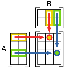
In order for the matrix product (\(A \times B\)) to exist, the number of columns in \(A\) must equal the number of rows in \(B\).
Basic properties of matrices
It is convention to represent vectors as column matrices. We are explicit in this representation in that we define two axes even through the number of columns is only one.
A column matrix in NumPy.
>>> x = np.array([[3,4,5,6]]).T
Note
Again notice the pair of double brackets
The .T indicates a transpose operation. In the case of
vectors we go from a rowwise representation to a columnwise one and
vice versa. We will spend more time on transposes in the next
section.
A row matrix in NumPy.
>>> x = np.array([[3,4,5,6]])
Since this is linear algebra essentials with the goal of preparing you for a learning experience in data science, lets introduce a running example that will help ground much of the notation and concepts.
Machine learning can be roughly split into two types of learning problems.
- Supervised learning - learn a mapping from inputs \(\mathbf{X}\) to outputs \(y\)
- Unsupervised learning - given only \(\mathbf{X}\), learn interesting patterns in \(\mathbf{X}\)
An example of this is to predict total snowfall, which would be a continuous \(\mathbf{y}\). When we use a feature matrix \(\mathbf{X}\) to predict \(\mathbf{y}\) it is an example of supervised learning. Our feature matrix would be a number of column vectors \(\mathbf{x}\) horizontally stacked together to form \(\mathbf{X}\). Examples of these features might be: the elevation, latitude, average winter temperature, historical snowfall data and more..
If we wanted to discover patterns in \(\mathbf{X}\) then we could take an such as clustering, which would be an example of unsupervised learning. Patterns in this case would likely correspond to mountain ranges and and meteorlogical or oceananic events..
If we think of the features of a matrix as column vectors.
>>> feature1 = np.array([[99,45,31,14]]).T
>>> feature2 = np.array([[0,1,1,0]]).T
>>> feature3 = np.array([[5,3,9,24]]).T
We can stack them into a matrix using hstack.
>>> X = np.hstack([feature1,feature2,feature3])
>>> X
array([[99,  0,  5],
       [45,  1,  3],
       [31,  1,  9],
       [14,  0, 24]])
There are easier ways to create matrices, such as reading directly
from a csv file, but the ability to concatenate matrices is important.
With hstack we horizontally stacked our column vectors. The
sister function vstack allows us to vertically stack vectors
or matrices in a similar way.
We may access the individual elements of \(\mathbf{X}\) through indexing
In the above matrix we show how to explicitly refer to any element in \(\mathbf{X}\). It is also quite common to refer to a generic element in \(\mathbf{X}\) as \(\mathbf{X}_{i,j}\), where if you picked up on the pattern indexing occurs by stating the row then the column. In NumPy you are following the same pattern. Using the feature matrix created above:
>>> X[0,2]
5
>>> X[1,0]
45
And if we want to access our first column vector again
>>> X[:,0]
array([99, 45, 31, 14])
>>> X[:,0]
array([99, 45, 31, 14])
We now see that an array with 2 axes is indexed and even sliced one axis at a time. 1D arrays can be indexed in the same way a Python list can.
>>> a = np.arange(10)
>>> a[2:4]
array([2, 3])
>>> a[:10:2]
array([0, 2, 4, 6, 8])
>>> a[::-1]
array([9, 8, 7, 6, 5, 4, 3, 2, 1, 0])
If we go back to the X matrix there are many useful functions once we are here including mean
>>> X.mean(axis=0)
array([ 47.25,   0.5 ,  10.25])
>>> X.mean(axis=1)
array([ 34.66666667,  16.33333333,  13.66666667,  12.66666667])
>>> X.mean()
19.333333333333332
Note
axis 0 refers to a mean with respect to the columns
Basic matrix operations
This has already been stated once. But since it is important lets say it a different way.
Note
In order to multiply two matrices, they must be conformable such that the number of columns of the first matrix must be the same as the number of rows of the second matrix.
When we say multiply two matrices it does not mean multiply in the sense that you might think. The matrix product of two matrices is another matrix.
If we have two vectors \(\mathbf{x}\) and \(\mathbf{y}\) of the same length \((n)\), then the dot product is give by
Important
Arithmetic operators in NumPy work elementwise
>>> a = np.array([3,4,5])
>>> b = np.ones(3)
>>> a - b
array([ 2.,  3.,  4.])
Something that can be tricky for people familar with other programming languages is that the * operator does not carry out a matrix product. This is done with the dot function.
>>> a = np.array([[1,2],[3,4]])
>>> b = np.array([[1,2],[3,4]])
>>> a
array([[1, 2],
       [3, 4]])
>>> b
array([[1, 2],
       [3, 4]])
>>> a * b
array([[ 1,  4],
       [ 9, 16]])
>>> np.dot(a,b)
array([[ 7, 10],
       [15, 22]])
>>> np.dot(np.array([[1,2,3]]),np.array([[2,3,4]]))
The dot product is a very important concept that we will reuse many times going forward. The dot product is generally written as
when you write np.dot the NumPy package will sometimes assume that you mean to do this such as in the case of the above example.
>>> np.dot(np.array([1,2,3,4]), np.array([3,4,5,6]))
50
>>> np.dot(np.array([[1,2,3,4]]), np.array([[3,4,5,6]]).T)
array([[50]])
The dot product is an essential building block of matrix multiplication. The table below shows that when we multiply two matrices the result is a table of dot products for pairs of vectors making up the entries of each matrix.
First think about this in terms of square matrices and see if you can identify the pattern.
Perform matrix multiplication on a square matrix. This is how it works—code the pattern.
Once you see what is happening this figure can help you understand how the pattern generalizes to different shap matrices. Figuring out the shape of a matrix that gets
https://en.wikipedia.org/wiki/Matrix_multiplication
Important
There is a pattern to figure out the size fo the resulting matrix. result = Num Rows in 1st matrix \(\times\) Num Columns in 2nd Matrix
Questions
Given the following code write the multiplication out on paper and run it Python to check your math
>>> np.dot(np.array([[1,2,3]]),np.array([[2,3,4]]).T)
If we multiply a \(2 \times 3\) matrix with a \(3 \times 1\) matrix, the product matrix is \(2 \times 1\).
Write an example of this on paper with simple numbers to see if you can understand why.
Khan academy video on dot products
Special addition and multiplication operators
Like in regular Python there is a special operator.
>>> a = np.zeros((2,2),dtype='float')
>>> a += 5
>>> a
array([[ 5.,  5.],
       [ 5.,  5.]])
>>> a *= 5
>>> a
array([[ 25.,  25.],
       [ 25.,  25.]])
>>> a + a
array([[ 50.,  50.],
       [ 50.,  50.]])
Sorting arrays
NumPy has a useful submodule to create random numbers
>>> x = np.random.randint(0,10,5)
>>> x.sort()
>>> x
array([0, 1, 5, 6, 7])
We can also reshuffle the array
>>> np.random.shuffle(x)
>>> x
array([1, 0, 6, 5, 7])
But sometimes we do not want to change our matrix, but knowing the sorted indices may be useful and here argsort can be very useful.
>>> sorted_inds = np.argsort(x)
>>> sorted_inds
array([1, 0, 3, 2, 4])
>>> x[sorted_inds]
array([0, 1, 5, 6, 7])
Common math functions
>>> x = np.arange(1,5)
>>> np.sqrt(x) * np.pi
array([ 3.14159265,  4.44288294,  5.44139809,  6.28318531])
>>> 2**4
16
>>> np.power(2,4)
16
>>> np.log(np.e)
1.0
>>> x = np.arange(5)
>>> x.max() - x.min()
4
There are so many mathematical functions available to you in NumPy
Basic operations exercise
Exercise
In the following table we have expression values for 5 genes at 4 time points. These are completely made up data. Although, some of the questions can be easily answered by looking at the data, microarray data generally come in much larger tables and if you can figure it out here the same code will work for an entire gene chip.
| Gene name | 4h | 12h | 24h | 48h |
|---|---|---|---|---|
| A2M | 0.12 | 0.08 | 0.06 | 0.02 |
| FOS | 0.01 | 0.07 | 0.11 | 0.09 |
| BRCA2 | 0.03 | 0.04 | 0.04 | 0.02 |
| CPOX | 0.05 | 0.09 | 0.11 | 0.14 |
- Create a single array for the data (4x4)
- Find the mean expression value per gene
- Find the mean expression value per time point
Extra Credit
- Which gene has the maximum mean expression value?
- Sort the gene names by the max expression value
Tip
>>> geneList = np.array([["A2M", "FOS", "BRCA2","CPOX"]])
>>> values0  = np.array([[0.12,0.08,0.06,0.02]])
>>> values1  = np.array([[0.01,0.07,0.11,0.09]])
>>> values2  = np.array([[0.03,0.04,0.04,0.02]])
>>> values3  = np.array([]0.05,0.09,0.11,0.14]])