Thinking in terms of vectors and matrices
| Learning Objectives | |
|---|---|
| 1 | Become familiar with linear algebra’s basic data structures: scalar, vector, matrix, tensor |
| 2 | Create, manipulate, and generally begin to get comfortable with NumPy arrays |
So you may be asking why?
Here are just a few reasons why a solid understanding of linear algebra is crutial for a practicing data scientist
- Linear models can concisly be written in vector notation
- Regularization often makes use of matrix norms
- Matrix decompsitions are commonly used in recommender systems
Scalars, vectors, matrices and tensors
Without knowing anything about vectors or matrices there is already a good chance that you have some intuition for these concepts. Think of a spreadsheet with rows and columns. Within a given cell there exists some value—lets call it a scalar; scalars are the contents of vectors and matrices. If we think of the idea of a column and the elements contained therein we now have a basis for the concept of a vector. More specifically, this is referred to as a column vector. The elements of a row are accordingly referred to as a row vector.
We collectively refer to the columns and rows as matrix.
Note
A matrix with \(m\) rows and \(n\) columns is a \(m \times n\) matrix and we refer to \(m\) and \(n\) as dimensions.
If a matrix is a two dimensional representation of data then a tensor is the generalization of that representation to any number of dimensions. Lets say we copied our spreadsheet and created several new tabs then we are now working with a tensor.
| Machine Learning | Notation | Description |
|---|---|---|
| Scaler | \(x\) | a single real number (ints, floats etc) |
| Vector | \(\mathbf{x}\) or \(\mathbf{x}^{T}\) | a 1D array of numbers (real, binary, integer etc) |
| Matrix | \(\mathbf{X}\) | a 2D array of numbers |
| Tensor | \(\hat{f}\) | an array generalized to n dimensions |
Matrices are also tensors. If we were working with a \(4 \times 4\) matrix it can be described as a tensor of rank 2. The rank is the formal term for the number of dimensions.
Questions
- So what are the dimensions of the following matrix
The matrix dimensions are \(3 \times 4\)
- Given a spreadsheet that has 4 tabs and each tab has 2 rows with 3 columns how might we represent that data with a tensor?
The tensor would be of rank 3 and have the following dimensions \(2 \times 3 \times 4\). In NumPy this is written as a \(4 \times 2 \times 3\). You will soon be working with NumPy and you can refer back to this example.
>>> x = np.array([[[ 0,  1,  2],
                   [ 3,  4,  5]],
                  [[ 9, 10, 11],
                   [15, 16, 17]],
                  [[ 2, 10, 8],
                   [5, 4, 9]],
                  [[18, 19, 20],
                   [24, 25, 26]]])
>>> print(x.shape)
(4, 2, 3)
Notation
Scalers have the standard math notation
\[x = 1\]
Vectors are denoted by lower case bold letters such as \(\mathbf{x}\), and all vectors are assumed to be column vectors.
\[\begin{split}\mathbf{x} = \begin{pmatrix} 0 \\ 1 \\ 2 \\ 3 \end{pmatrix}\end{split}\]
A superscript \(T\) denotes the transpose of a matrix or vector. This implies that \(\mathbf{x}^{T}\) is a row vector.
\[\mathbf{x}^{T} = \begin{pmatrix} 0 & 1 & 2 & 3 \end{pmatrix}\]
Upper-case bold letter denote.
\[\begin{split}\mathbf{X} = \begin{pmatrix} 0 & 0 & 1 & 0 \\ 1 & 2 & 0 & 1 \\ 1 & 0 & 0 & 1 \end{pmatrix}\end{split}\]
An introduction to NumPy and Arrays
Sometimes we need to write concepts on paper or see them in action through code before we can effectively establish our understanding. We will be learning the through a widely used Python package called NumPy to help bring to life the essentials of linear algebra.
In order to get the most out of this resource and to ensure that you can actively follow along it is easiest if you install a working Python environment.
Important
Familiarity with the Python language is not a prerequisite for this primer. The included code blocks are minimal and you should be able to follow even without prior experience in Python.
Once Python is installed you can start an interactive Python
environment by typing the command ipython into a terminal. NumPy is the de facto standard for numerical computing
in Python and it comes installed as part of the Conda bundle. It is
highly optimized and
extremely useful for working with matrices. The standard matrix class
in NumPy is called an array.
We will first get comfortable working with arrays then we will ease
our way into the essential concepts of linear algebra. NumPy will
provide you with a tool explore all concepts presented here.
The standard syntax for importing the package NumPy into a Python environment is
>>> import numpy as np
Note
Examples of code (like the import statement above) are line by line, where each line begins with >>>. This means that you can copy the code that comes after the line indicator directly into your interpreter
Arrays and their attributes
Python is an object-oriented programming language. The main object in NumPy is the homogeneous, multidimensional array. An array is our programmatic way to represent vectors and matrices. An example is a matrix \(\mathbf{X}\)
and can be represented through NumPy as
>>> import numpy as np
>>> X = np.array([[1,2,3],[4,5,6],[7,8,9]])
>>> X
array([[1, 2, 3],
       [4, 5, 6],
       [7, 8, 9]])
Lets break down that code statement. First
>>> a = [1,2,3]
is a native Python data structure called a list. We could create a vector from this list using the NumPy array class.
>>> a = np.array([1,2,3])
So to create the above X matrix it is a list of lists where each row corresponds to a list.
Because our array version of \(\mathbf{X}\) is an object it contains methods and attributes.
- The methods are functions that act on our matrix
- the attributes are data that are related to our matrix.
Lets start with some useful attributes. The array \(\mathbf{X}\)
has 2 dimensions. The number of dimensions in linear algebra
terminology is referred to as rank. We get at rank with the
ndim attribute.
>>> X.ndim
2
similarly we have access to the dimensions themselves through shape
>>> X.shape
(3, 3)
Note that the number of axes is also equal to the or the length of x.shape. To return an integer representing the total number of elements one may use size.
>>> X.size
9
Warning
If you want to work with a vector where the dimensions exist explicitly you need to use double brackets. Otherwise it will be a 1D matrix and sometimes it may not give you the result you were looking for.
>>> np.array([1,2,3]).shape
(3,)
>>> np.array([[1,2,3]]).shape
(1, 3)
Arrays and their methods
We have seen that arrays have built in attributes that are useful. They also have numerous built-in methods that make them particularly convenient. Note that methods always have parenthesis that may or may not enclose arguments.
>>> X.sum(axis=0)
array([12, 15, 18])
>>> X.sum(axis=1)
array([ 6, 15, 24])
>>> X.mean(axis=0)
array([ 4.,  5.,  6.])
>>> X.mean(axis=1)
array([ 2.,  5.,  8.])
Commonly used arrays can be created with functions that are part of the NumPy package. For example, to make a sequence of numbers, we can use arange. This is similar to the standard python function range that returns a list instead of an array. Look carefully at the following examples to see how it works.
>>> np.arange(10)
array([0, 1, 2, 3, 4, 5, 6, 7, 8, 9])
>>> np.arange(5,10)
array([5, 6, 7, 8, 9])
>>> np.arange(5,10,0.5)
array([ 5. ,  5.5,  6. ,  6.5,  7. ,  7.5,  8. ,  8.5,  9. ,  9.5])
Also we can recreate the first matrix by reshaping the output of arange.
>>> X = np.arange(1,10).reshape(3,3)
>>> X
array([[1, 2, 3],
       [4, 5, 6],
       [7, 8, 9]])
In that function we created an array with values from 1-10 then we reshaped it into a 2D array with 3 columns and 3 rows. Another similar function to arange is linspace which fills a vector with evenly spaced variables for a specified interval.
>>> x = np.linspace(0,5,5)
>>> x
array([ 0.  ,  1.25,  2.5 ,  3.75,  5.  ])
As a reminder you may access the Python documentation at anytime from the command line using
~$ pydoc numpy.linspace
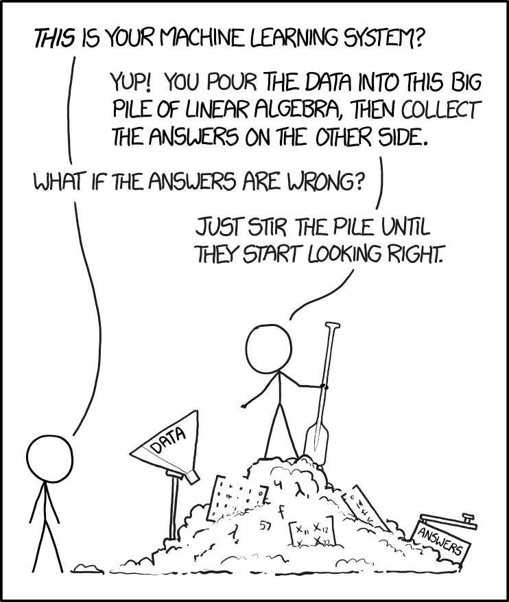
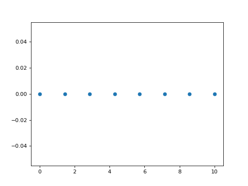
The following plot visualizes linspace. It is an important function, but it less important that you understand the plotting portion of the code.
import numpy as np
import matplotlib.pyplot as plt
fig = plt.figure()
ax = fig.add_subplot(111)
N = 8
y = np.zeros(N)
x1 = np.linspace(0, 10, N, endpoint=True)
p1 = plt.plot(x1, y, 'o')
ax.set_xlim([-0.5,10.5])
plt.show()
(Source code, png, hires.png, pdf)

Important
Did you notice that arange starts counting at zero?
Python uses zero based indexing, so the initial element
of a sequence has index 0.
This is a good time to introduce the idea that arrays may be made of different types of data, but they can only be one data type at a given time.
>>> x = np.array([1,2,3])
>>> x.dtype
dtype('int64')
>>> x = np.array([0.1,0.2,0.3])
>>> x
array([ 0.1,  0.2,  0.3])
>>> x.dtype
dtype('float64')
>>> x = np.array([1,2,3],dtype='float64')
>>> x.dtype
dtype('float64')
There are several convenience functions for making arrays that you should be aware of:
>>> x = np.zeros([3,4])
>>> x
array([[ 0.,  0.,  0.,  0.],
       [ 0.,  0.,  0.,  0.],
       [ 0.,  0.,  0.,  0.]])
>>> x = np.ones([3,4])
>>> x
array([[ 1.,  1.,  1.,  1.],
       [ 1.,  1.,  1.,  1.],
       [ 1.,  1.,  1.,  1.]])
Exercise
- Create the following matrix using a NumPy array (1 line)
>>> a = np.arange(1,101).reshape(10,10)
- Use the array object to get the rank, number of elements, and dimensions
>>> print("Rank: {}\nSize: {}\nDimensions: {}".format(a.ndim,a.size,a.shape))
Rank: 2
Size: 100
Dimensions: (10, 10)
- Get the mean of the rows and columns
>>> print("Row means: {}".format(a.mean(axis=1)))
Row means: [  5.5  15.5  25.5  35.5  45.5  55.5  65.5  75.5  85.5  95.5]
>>> print("Column means: {}".format(a.mean(axis=0)))
Column means: [ 46.  47.  48.  49.  50.  51.  52.  53.  54.  55.]
- How do you create a vector that has exactly 50 points and spans the range 11 to 23?
>>> b = np.linspace(11,23,50)
[extra] If you want a peak at whats to come see what happens when you do the following
- np.log(a)
- np.cumsum(a)
- np.power(a,2)