Linear Algebra Part II

These concepts build on what we learned in part I

Learning Objectives
1	Understand some applications of and basic fundamentals of norms
2	Extend the concept of a norm to cosine similarity
3	Develop a familiarity with systems of equations and their linear algebra shorthand

Norms and other special matrices

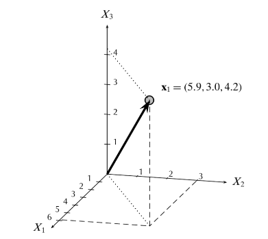
Sometimes it is necessary to quantify the size of a vector. There is a specific function called a called a norm that serves this purpose.

Here is an example of norm of a vector \(\mathbf{x}\) is defined by

\[||\mathbf{x}|| = \sqrt{x_1^2 + x_2^2 + \cdots + x_n^2}\]

>>> x = np.array([1,2,3,4])
>>> print(np.sqrt(np.sum(x**2)))
>>> print(np.linalg.norm(x))
5.47722557505
5.47722557505

The norm shown above is also known as Frobenius norm. The Frobenius norm, sometimes also called the Euclidean norm (a term unfortunately also used for the vector-norm), is norm of an matrix defined as the square root of the sum of the absolute squares of its elements. The following is a generalized way to write many types of norms.

\[||\mathbf{x}||_{p} = \left( \sum_{i} |x_i|^{p} \right)^{\frac{1}{p}}\]

• Norms are used to map vectors to non-negative values
• The Euclidean norm (where \(p=2\) ) of a vector measures the distance from the origin in Euclidean space

There are many nice properties of the Euclidean norm. The norm squared of a vector is just the vector dot product with itself

\[||x||^2 = x \cdot x\]

>>> print(np.linalg.norm(x)**2)
>>> print(np.dot(x,x))
30
30

Important

The distance between two vectors is the norm of the difference.

\[d(x,y) = ||x-y||\]

>>> np.linalg.norm(x-y)
4.472

Cosine Similarity is the cosine of the angle between the two vectors give by

\[cos(\theta) = \frac{\mathbf{x} \cdot \mathbf{y}}{||\mathbf{x}|| \text{ } ||\mathbf{y}||}\]

>>> x = np.array([1,2,3,4])
>>> y = np.array([5,6,7,8])
>>> np.dot(x,y)/(np.linalg.norm(x)*np.linalg.norm(y))
0.96886393162696616

If both \(\mathbf{x}\) and \(\mathbf{y}\) are zero-centered, this calculation is the correlation between \(\mathbf{x}\) and \(\mathbf{y}\).

>>> from scipy.stats import pearsonr
>>> x_centered = x - np.mean(x)
>>> y_centered = y - np.mean(y)
>>> r1 = np.dot(x_centered,y_centered)/(np.linalg.norm(x_centered)*np.linalg.norm(y_centered))
>>> r2 = pearsonr(x_centered,y_centered)
>>> print(r1,r2[0])
1.0 1.0

Special matrices

Let \(X\) be a matrix of dimension \(n \times k\) and let \(Y\) be a matrix of dimension \(k \times p\), then the product \(XY\) will be a matrix of dimension \(n \times p\) whose \((i,j)^{th}\) element is given by the dot product of the \(i^{th}\) row of \(X\) and the \(j^{th}\) column of \(Y\)

\[\sum_{s=1}^k x_{is}y_{sj} = x_{i1}y_{1j} + \cdots + x_{ik}y_{kj}\]

Orthogonal Matrices

Let \(X\) be an \(n \times n\) matrix such than \(X^TX = I\), then \(X\) is said to be orthogonal which implies that \(X^T=X^{-1}\)

This is equivalent to saying that the columns of \(X\) are all orthogonal to each other (and have unit length).

System of equations

A system of equations of the form:

\[\begin{split}\begin{align*} a_{11}x_1 + \cdots + a_{1n}x_n &= b_1 \\ \vdots \hspace{1in} \vdots \\ a_{m1}x_1 + \cdots + a_{mn}x_n &= b_m \end{align*}\end{split}\]

can be written as a matrix equation:

\[A\mathbf{x} = \mathbf{b}\]

and hence, has solution

\[\mathbf{x} = A^{-1}\mathbf{b}\]

Additional Properties of Matrices

1. If \(X\) and \(Y\) are both \(n \times p\) matrices,then

   \[X+Y = Y+X\]

2. If \(X\), \(Y\), and \(Z\) are all \(n \times p\) matrices, then

   \[X+(Y+Z) = (X+Y)+Z\]

3. If \(X\), \(Y\), and \(Z\) are all conformable,then

   \[X(YZ) = (XY)Z\]

4. If \(X\) is of dimension \(n \times k\) and \(Y\) and \(Z\) are of dimension \(k \times p\), then

\[X(Y+Z) = XY + XZ\]

5. If \(X\) is of dimension \(p \times n\) and \(Y\) and \(Z\) are of dimension \(k \times p\), then

\[(Y+Z)X = YX + ZX\]

6. If \(a\) and \(b\) are real numbers, and \(X\) is an \(n \times p\) matrix, then

   \[(a+b)X = aX+bX\]

7. If \(a\) is a real number, and \(X\) and \(Y\) are both \(n \times p\) matrices,then

   \[a(X+Y) = aX+aY\]

8. If \(z\) is a real number, and \(X\) and \(Y\) are conformable, then

   \[X(aY) = a(XY)\]

Another resource is this Jupyter notebook that review much of these materials

• ../notebooks/linear-algebra.ipynb